
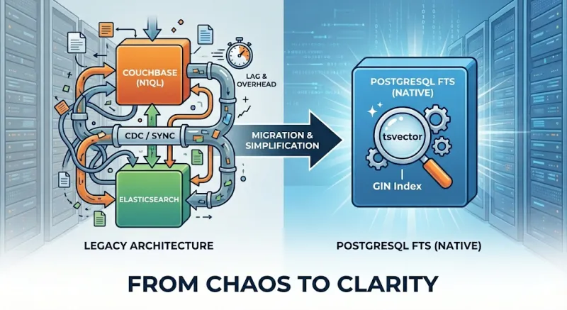
Adding full-text search to an application usually means spinning up Elasticsearch, OpenSearch, or Solr. That approach works, but it introduces another system to run, sync, and keep consistent. We challenged that assumption and ended up replacing Elasticsearch with PostgreSQL's built-in full-text search. This article shares our journey and a practical guide to using PostgreSQL FTS.
Who Should Read This
Engineers and architects considering search solutions for medium-scale applications will find this useful. If you already use PostgreSQL and your search volume is moderate—hundreds of thousands to a few million documents, tens to low hundreds of queries per second—PostgreSQL Full Text Search may be enough. We cover the trade-offs and a step-by-step tutorial to evaluate it for your own use case.
Why consider PostgreSQL FTS before Elasticsearch? As Miftahul Huda notes, Elasticsearch is often overkill for small-to-medium apps. It requires additional expertise, complex deployment and monitoring, extra operational cost, and synchronization between your primary database and the search index. PostgreSQL's built-in search provides language support, simpler architecture, cost efficiency, and zero sync lag—all without extra infrastructure.
Our Search Journey
The Problem: Couchbase and N1QL
Couchbase was our primary document store. We relied on it with N1QL for queries. In production, we ran into N1QL performance limits: query latency increased under load, and some search patterns were hard to optimize. We needed a dedicated search layer that could handle text search efficiently.
First Attempt: CDC to Elasticsearch
We built and adopted go-dcp-elasticsearch, which streams Couchbase documents to Elasticsearch via the Database Change Protocol (DCP). It performed well and reduced search latency, but it introduced several problems:
- Synchronization and refresh delays. Elasticsearch's refresh interval means documents are not immediately searchable after indexing. Users often did not see their own just-written changes (read-your-writes consistency was broken), which was unacceptable for our product flows.
- DCP protocol constraints. The DCP stream only carries the latest state per document. If indexing a document to Elasticsearch failed, we had no way to replay that change. We either had to process vbucket events without blocking ( and accept possible data loss) or persist failed documents somewhere for retry.
- Additional system to operate. We now had to run, monitor, and scale another service (the connector) plus Elasticsearch itself. Failures in the pipeline directly affected search freshness and correctness.
The Turning Point: PostgreSQL Migration
Our document model—relational entities, clear schemas, and transactional updates—fits PostgreSQL better than Couchbase. We planned a migration to PostgreSQL, which raised a key question: should we keep Elasticsearch for search?
Keeping it would mean another CDC pipeline, this time from PostgreSQL to Elasticsearch. We had go-pq-cdc-elasticsearch for this purpose, which streams PostgreSQL changes to Elasticsearch via logical replication. It solves the Couchbase-specific DCP replay limitation, but the fundamental challenges remain: Elasticsearch is eventually consistent, and the connector is another moving part to run and debug.
Our Staff Engineer, Nurettin Bakkal, suggested we evaluate PostgreSQL Full Text Search first. Our workload—moderate data size and query volume—made this approach plausible. We ran a POC and the results were strong enough to adopt PostgreSQL FTS as our primary search solution.
LIKE, Regex, and Full-Text Search: Why They're Different
Like many developers, our initial approach to implementing search functionality in databases was refreshingly simple, if not a bit naive:
SELECT * FROM products
WHERE overview LIKE '%keyboard%';
We would sprinkle in some wildcards, maybe throw in a case-insensitive ILIKE operator, and call it a day. When
requirements got more specific, we'd reach for regular expressions, feeling quite clever about patterns like:
SELECT * FROM products
WHERE overview ~* '\\ykeyboard\\y';
This approach worked fine for small projects and simple search requirements. However, reality hit hard when we encountered our first real-world search challenge.
What LIKE and regex cannot do:
- Stemming:
LIKE '%running%'won't match "run" or "ran"; you need separate patterns for each word form. - Stop words: Queries like "the best keyboard" still scan rows containing "the" and "best", adding noise and slowing scans.
- Ranking: Every match is treated equally; you get no relevance scoring.
- Index efficiency: B-tree indexes work for
LIKE 'word%'(prefix match) but not for'%word%'; the latter forces full-table scans. Regex behaves similarly.
What PostgreSQL Full-Text Search adds:
- Lexemes: Text is normalized (lowercased, stemmed, stop words removed) into searchable tokens.
- tsvector: Pre-computed, indexed representation of document content with positions and weights for ranking.
- tsquery: Structured queries with AND, OR, NOT, and phrase operators.
- GIN index: Enables fast lookups instead of full-table scans.
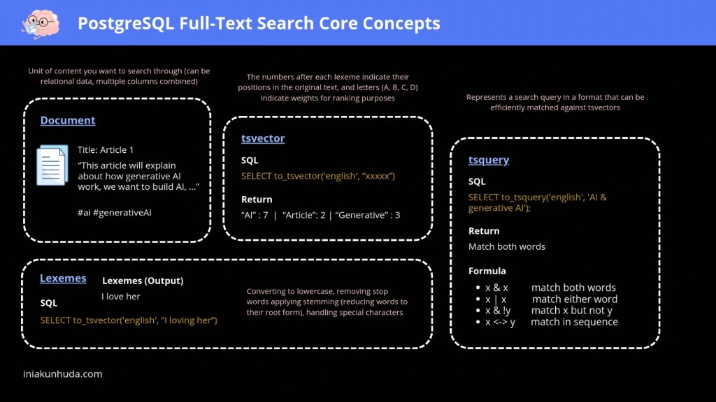
The diagram below summarizes how documents become tsvectors and how tsquery enables efficient, ranked search:
PostgreSQL Full Text Search: A Practical Guide
This section is a hands-on reference for implementing PostgreSQL FTS. If you are reading this as a presentation, feel free to skip ahead to the Conclusion—you can return here when you are ready to implement.
It is based on Adam Cooper's excellent posts, Miftahul Huda's practical guide, and the PostgreSQL documentation.
tsvector and to_tsvector
A tsvector is a sorted list of distinct lexemes—normalized tokens used for matching. to_tsvector turns raw text
into a tsvector:
SELECT to_tsvector('I am altering the deal. Pray I do not alter it further!');Output: 'alter':3,10 'deal':5 'further':12 'pray':6 (stop words like "I", "am", "the" are removed; words are stemmed
and positions preserved).
tsquery and Matching
A tsquery represents a search condition. Use @@ to check if a tsvector matches a tsquery:
SELECT title FROM movies WHERE to_tsvector(title) @@ to_tsquery('star');tsquery requires operator-separated tokens. Plain text like 'star wars' is invalid. Use plainto_tsquery to build a
query from user input:
SELECT title, ts_rank(to_tsvector(title), plainto_tsquery('star wars')) AS rank
FROM movies
WHERE to_tsvector(title) @@ plainto_tsquery('star wars')
ORDER BY rank DESC;
websearch_to_tsquery: User-Friendly Syntax
websearch_to_tsquery supports a simple, familiar syntax:
"quoted text"→ phrase match (terms in order)-→ NOTOR→ OR- Unquoted terms are ANDed by default
For programmatic phrase queries, phraseto_tsquery builds a tsquery that requires terms to appear in sequence.
Example: search for "star wars" but exclude "clone":
SELECT title, ts_rank(title_search, websearch_to_tsquery('"star wars" -clone')) AS rank
FROM searchable_docs
WHERE title_search @@ websearch_to_tsquery('"star wars" -clone')
ORDER BY rank DESC;
Multi-Column Search with setweight
Use setweight to give different columns different importance (A highest, D lowest):
SELECT setweight(to_tsvector(title), 'A') || setweight(to_tsvector(overview), 'B')
FROM searchable_docs;
Generated Columns for tsvector
Instead of computing tsvector at query time, store it in a generated column so the vector is built once at write
time—just like Elasticsearch indexes documents on ingestion. This shifts the cost from read to write, enabling fast
searches via the pre-computed column and GIN index:
ALTER TABLE searchable_docs
ADD COLUMN title_search tsvector
GENERATED ALWAYS AS (
    setweight(to_tsvector('simple', coalesce(title, '')), 'A') ||
    setweight(to_tsvector('simple', coalesce(overview, '')), 'B') ||
    setweight(to_tsvector('simple', coalesce(tags, '')), 'C')
) STORED;
Use coalesce to handle NULL columns—to_tsvector(NULL) returns NULL and would break the expression;
coalesce(title, '') guarantees a string. Use the 'simple' text search config so the expression is immutable (
generated columns require this); language configs like 'english' depend on locale and dictionaries that can change.
With this approach, every INSERT and UPDATE automatically recomputes the tsvector—your application never needs to
manage indexing separately.
GIN Index for Performance
Without an index, full-text search does a sequential scan. Add a GIN index on the tsvector column:
CREATE INDEX idx_search ON searchable_docs USING GIN(title_search);This reduces query time from tens of milliseconds to well under a millisecond for typical datasets.
How GIN Index Works Internally
GIN (Generalized Inverted Index) is specifically designed for composite values—values that contain multiple elements,
like a tsvector containing multiple lexemes. Understanding its internal structure helps explain why full-text search
becomes so fast.
A GIN index has three core components:
Entry Tree (B-Tree of lexemes): The top-level structure is a regular B-Tree where each key is a distinct lexeme
extracted from all indexed tsvector values. When PostgreSQL builds a GIN index on a tsvector column, it collects
every unique lexeme across all rows and inserts them into this B-Tree. This allows O(log n) lookup for any lexeme.
Posting List: For lexemes that appear in a small number of rows, GIN stores a simple sorted array of TIDs (Tuple IDs—pointers to heap rows) directly alongside the lexeme in the Entry Tree. This is compact and fast for low-frequency terms.
Posting Tree: When a lexeme appears in many rows and the TID list grows beyond a threshold, GIN promotes the flat list into a separate B-Tree of TIDs—the Posting Tree. This keeps lookups efficient even for very common terms, since searching a B-Tree of TIDs is O(log n) rather than scanning a long flat list.
Let's walk through a concrete example. Suppose we have a table with a tsvector column called icerik and we run:
SELECT * FROM documents
WHERE icerik @@ to_tsquery('elma & tatlı')
ORDER BY ts_rank(icerik, to_tsquery('elma & tatlı')) DESC;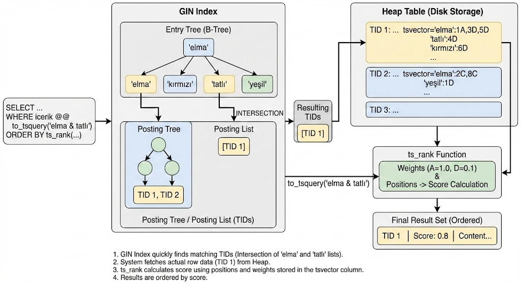
Here is what happens step by step:
1. Entry Tree lookup: PostgreSQL looks up both 'elma' and 'tatlı' in the Entry Tree (B-Tree). This is a standard
B-Tree traversal—O(log n) for each lexeme.
2. Choosing the smaller set first: The query optimizer starts with the less frequent term. If 'tatlı' appears in
fewer documents than 'elma', PostgreSQL fetches 'tatlı''s TID set first. Since 'tatlı' has few matching rows, its
TIDs are stored as a Posting List (flat sorted array): e.g. [TID 1].
3. Intersection via the Posting Tree: Now PostgreSQL needs to intersect this with 'elma''s matches. 'elma'
appears in many documents, so its TIDs are stored in a Posting Tree (B-Tree of TIDs). Instead of loading all of
'elma''s TIDs, PostgreSQL takes each TID from 'tatlı''s small list and probes 'elma''s Posting Tree—a O(log n)
lookup per TID. This is far cheaper than intersecting two large flat lists.
4. Heap fetch: The resulting TIDs (e.g. [TID 1]) point directly to rows in the heap table. PostgreSQL fetches the
actual row data, including the stored tsvector with position and weight information.
5. Ranking: ts_rank uses the position and weight metadata stored in the tsvector column (e.g.
'elma':1A,3D,5D 'tatlı':4D) to calculate a relevance score. Weights A through D (A=1.0, B=0.4, C=0.2, D=0.1 by
default) determine how much each match contributes.
6. Result ordering: Results are sorted by score descending. A document where 'elma' appears in an A-weighted field
scores higher than one where it only appears in D-weighted fields.
The key insight is the asymmetry: by starting with the rarer term and probing the common term's Posting Tree, GIN avoids materializing large intermediate result sets. This is what makes GIN-backed full-text search fast even when individual lexemes match thousands of rows.
Text Search Configuration
PostgreSQL uses text search configurations for language-specific behavior. simple lowercases and removes a minimal set
of stop words. Language configs (e.g. english) add stemming:
SELECT to_tsvector('english', 'To fish the fishes a fishy fisher fished');Output: 'fish':2,4,6,7,8 (all forms normalized to "fish"; stop word positions 1, 3, 5 are skipped).
PostgreSQL also supports turkish for Turkish text:
SELECT to_tsvector('turkish', 'Türkiye''nin en büyük e-ticaret platformunda arama yapıyoruz');Output: 'ara':6 'büyük':3 'e-ticaret':4 'platform':5 'türkiy':1 'yap':7 (Turkish stop words "nin", "en", "da" are
removed; suffixes are stripped by the Turkish stemmer).
ts_rank Normalization
By default, ts_rank does not account for document length. Short documents that match exactly can rank lower than
longer ones. Use the normalization parameter:
SELECT title, ts_rank(title_search, websearch_to_tsquery('rush'), 1) AS rank
FROM searchable_docs
WHERE title_search @@ websearch_to_tsquery('rush')
ORDER BY rank DESC;
The third argument 1 divides the rank by 1 + log(document length), improving ranking for short, exact matches.
ts_headline: Highlighting Matches in Results
Use ts_headline to return a snippet of matching content with search terms wrapped for highlighting:
SELECT title,
  ts_headline('english', overview, websearch_to_tsquery('postgresql'),
    'StartSel=<mark>, StopSel=</mark>, MaxFragments=1, MaxWords=50, MinWords=20') AS snippet
FROM searchable_docs
WHERE title_search @@ websearch_to_tsquery('postgresql')
ORDER BY ts_rank(title_search, websearch_to_tsquery('postgresql')) DESC;
This returns a single fragment of 20–50 words with matches wrapped in <mark> tags, useful for search result previews.
Extensions: pg_trgm and unaccent
For fuzzy search (typo tolerance) and diacritic handling:
CREATE EXTENSION IF NOT EXISTS pg_trgm;   -- Trigram similarity, e.g. similarity('keybord', 'keyboard')
CREATE EXTENSION IF NOT EXISTS unaccent;  -- Removes diacritics: 'café' matches 'cafe'
pg_trgm enables % and <-> operators for similarity matching; unaccent helps with international content.
Complete Example
CREATE TABLE products (
    id SERIAL PRIMARY KEY,
    title TEXT NOT NULL,
    overview TEXT,
    tags TEXT,
    search_vector tsvector GENERATED ALWAYS AS (
        setweight(to_tsvector('simple', coalesce(title, '')), 'A') ||
        setweight(to_tsvector('simple', coalesce(overview, '')), 'B') ||
        setweight(to_tsvector('simple', coalesce(tags, '')), 'C')
    ) STORED
);

CREATE INDEX idx_products_search ON products USING GIN(search_vector);

SELECT id, title, ts_rank(search_vector, websearch_to_tsquery('premium wireless')) AS rank
FROM products
WHERE search_vector @@ websearch_to_tsquery('premium wireless')
ORDER BY rank DESC
LIMIT 20;
Conclusion
PostgreSQL Full Text Search was the right choice for us. We eliminated an entire layer of infrastructure—Elasticsearch, CDC connectors, and the operational burden that came with them—and replaced it with a feature already built into our primary database.
What we gained:
- Strong consistency: No sync lag; read-your-writes by default. Every INSERT is immediately searchable.
- Simpler architecture: One database instead of PostgreSQL + Elasticsearch + CDC pipeline.
- Lower operational load: Fewer services to run, monitor, and debug at 3 AM.
- Good performance: At our moderate scale, both read and write latency are well within requirements. Elasticsearch returned at p50 35ms; PostgreSQL at p50 45ms. Since this was a low-traffic endpoint where we could tolerate the 10ms difference, the trade-off was acceptable. The tsvector is computed at insert time via a generated column—lightweight and efficient.
PostgreSQL FTS is not a replacement for Elasticsearch in every scenario. While PostgreSQL's full-text search is powerful, Elasticsearch may be the better choice when:
- Your data volume exceeds several million records
- You need distributed search across multiple nodes
- You require complex aggregations and analytics
- Your search load exceeds thousands of queries per second
For moderate scale and consistency needs, PostgreSQL Full Text Search is a powerful, built-in alternative. Before adding another system to your stack, evaluate the one you already have.